Author’s Note: This is a blog post doing initial, informal exploration of the “Bad Hands” phenomenon. I would eventually like to write a paper about this, but for now just consider this as a quick look.

Since the inception of diffusion-based image generation in 2021, one of the most recurring criticisms has been their tendancy to generate deformed human bodies, in particular, hands. Early theories about the hands problem included the following ideas:

1. Diffusion models basically just stitch together patches of images they’ve already seen, so they don’t actually know anything about hands
2. Models aren’t trained on enough hand data to be able to extrapolate all the possible hand positions
3. Models are trained on things like cartoons, where people might have 4 fingers, and things like body horror, where people’s fingers might melt into other stuff, so they think that there’s some leeway in how hands can be.

Enough time has passed that all of these theories can be debunked:

1. Diffusion models contain meaningful and useful world models
2. Modern models like flux have been extensively trained on huge amounts of hand data specifically to counteract this problem, and yet we can still find some bad hands in flux, even in simple positions
3. If this was true, then it would be solved simply by filtering the dataset. It would also show up very visibly in a linear probe!

We will investigate this problem in the context of Flux.1-dev, a large and popular open-weight model. Flux.1-dev uses basically all of the most modern architectures and features of other models, and it’s probably the most widely used open-weight model. In the vein of recent interpretability methods that have been applied to LLMs, we will look at the internal token representations at various layers and timesteps, and see what sort of structures emerge regarding the representation of hands.

Dataset

Before we can analyze any tokens, we need to collect a dataset. We want to label tokens as “good hand”, “bad hand”, or “not hand”. We adopt the convention that if any part of a hand is significantly deformed (including extra fingers), the entire hand is considered “bad”. ¹ Our dataset creation process consists of the following

1. Create a diverse set of prompts, that will show hands in a variety of styles, settings, scales, and positions.
   We used Claude Sonnet 3.7 to generate a long list of prompts that would satisfy this criteria.
2. Generate images from these prompts, and save the (seed, prompt) pair corresponding to each image. We used the Diffusers library and generated 500 images at 1024x1024 resolution, with 20 diffusion steps per image.
3. Label patches within the generated images. We created a simple webapp to quickly load images, and “draw” good/bad labels onto the patch grid of the image. We found that around 20% of images generated contained bad hands, so we tagged all of these images and an equal number of good-hand images. In total, we tagged around 200 images, corresponding to around 16,000 hand tokens.
4. Run the generation again with the same seeds and prompts, and save the intermediate activations for the hand tokens at selected timestamps and layers.

We choose to extract tokens at double block 12, and single blocks 8, 12, 16, 24, and 32; and timesteps 20, 19, 18, 17, 15, 12, 8, and 3 (that is, we focus more on the timesteps with higher noise levels).

Data Exploration

Prior work on large language model interpetability suggests that semantically meaningful directions tend to be consistent throughout layers. In other words, if the DiT’s “world model” includes an idea of good and bad hands, we’d expect a single direction (or small number of directions) to capture most of the information. However let’s start by just doing a PCA per block/timestep over the dataset.

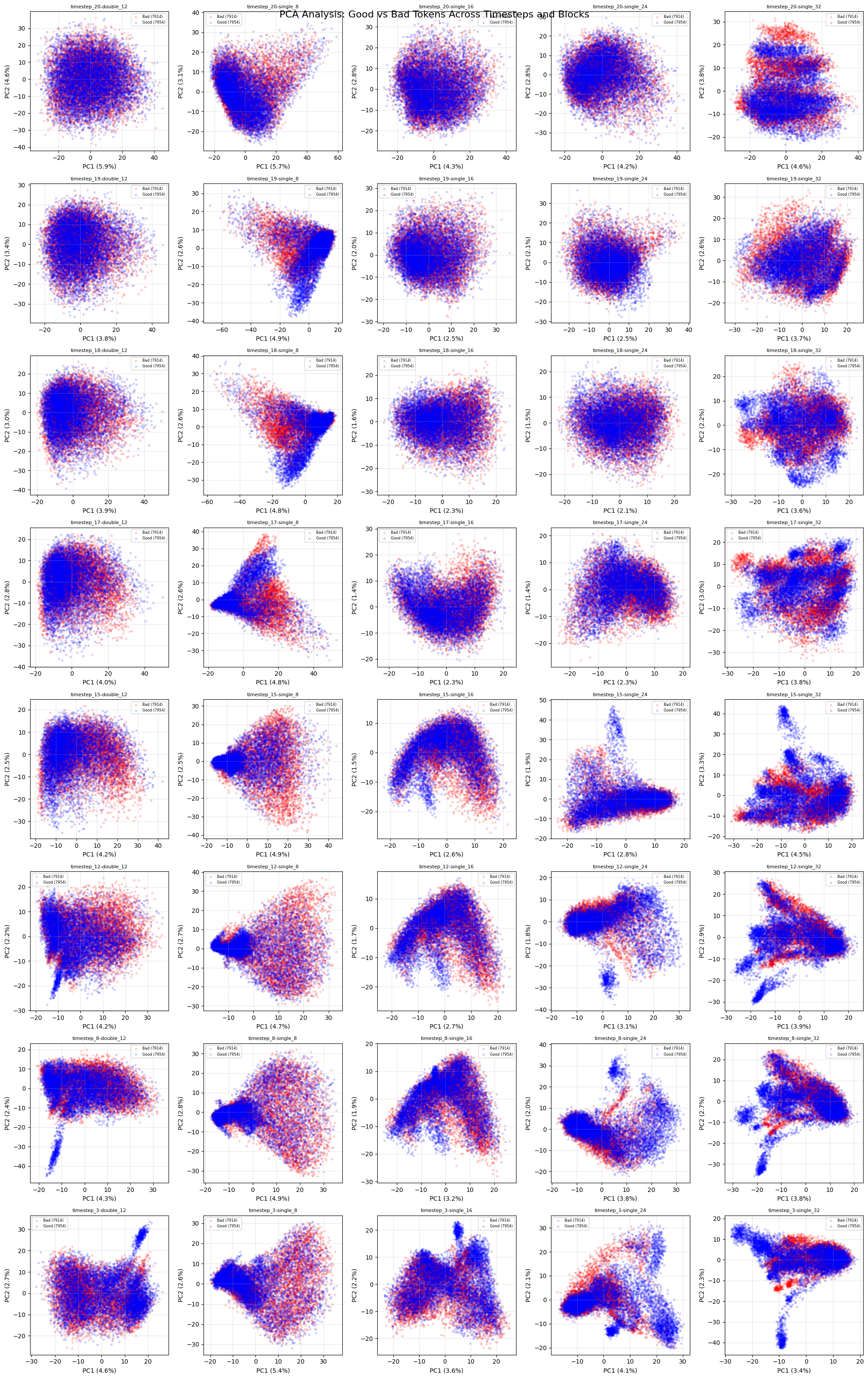
We note the following conclusions:

1. The good/bad distributions are not easily separated by PCA.
2. Activation structures become substantially less linear at later blocks
3. Activation structures are slightly less linear at later timesteps.
4. Single Block 8 contains much more variable structures than other early/middle blocks.

However, the fact that the PCA doesn’t reveal the structure we want doesn’t mean it isn’t there. After all, the variance of the dataset due to the differences in image content could be larger than the variance across the good/bad axis. So let’s try to explicitly separate by the good/bad axis. Letting \(\bar U_{i, t}^+\) and \(\bar U_{i, t}^-\) be the mean vector over the good and bad hand tokens (respectively) at block \(i\) and timestep \(t\), we can define \(v_{i, t} = \bar U_{i, t}^+ - \bar U_{i, t}^i\).

Let’s plot the per-block/timestep activations again, but this time we’ll put \(v_{i, t}\) as the x-axis, and then find the orthogonal direction to \(v_{i, t}\) with the highest variance, setting that as the y-axis. In other words, PCA against \(v_{i, t}\).

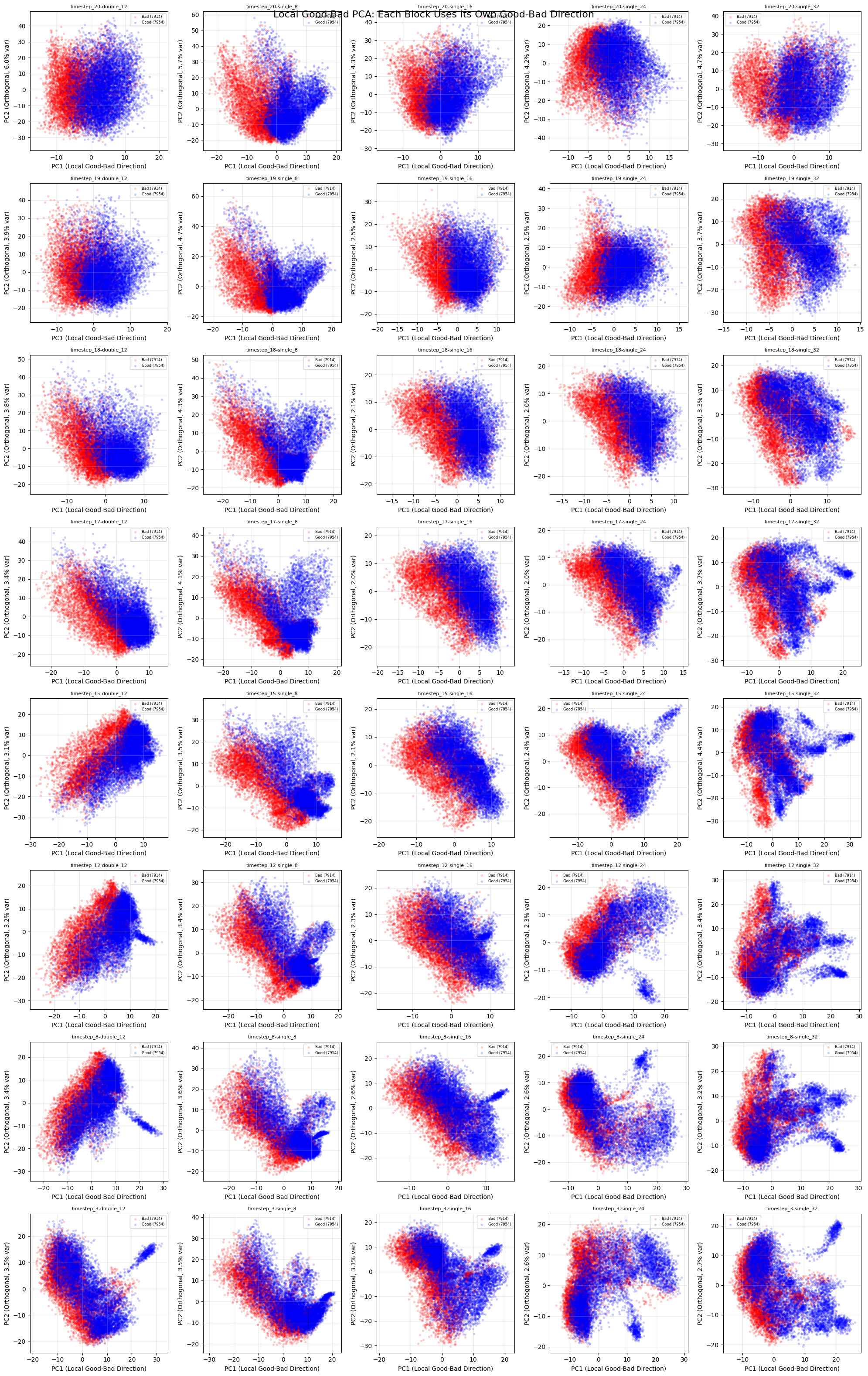
Conclusions from this graph:

1. We can separate the distributions much better now, although there’s still a substantial overlap.
2. Higher timesteps show a clearer separation between good and bad hands.
3. Block single-8 shows the clearest separation.

At this point, we should expect to be able to separate the two distributions reasonably well, at least at the block level. Before we go on to look for a global good-bad direction or attempt to create a classifier, let’s formalize this intuition. We want to measure the difference between the two distributions. For this we will use the Bhattacharyya Distance. Given two random variables \(P\) and \(Q\), with densities \(p(x)\) and \(q(x)\) respectively, define

and

The Bhattacharyya Coefficient \(BC\) is a measure of similarity and the Bhattacharyya Distance \(D_B\) is a measure of distance (note that it is not a metric…). Why do we use \(D_B\) over any number of other distance functions on probability measures? The answer is that \(D_B\) is related to the Bayes error rate, which is the lowest possible error of a binary classifier on the joint distribution. Moreover, if we model each token activation distribution as a diagional Gaussian (note that we don’t have enough data for a nondegenerate estimation of the full covariance matrix), we can efficiently compute \(D_B\) in closed form.

If we compute \(D_B\) per block/timestep, we have the following plot:

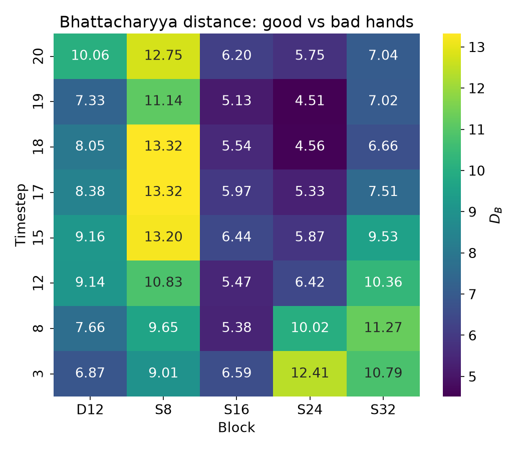
This confirms that the signal is strongest (out of the blocks we are considering) in Single Block 8 in early timesteps, but that it is lost later in the diffusion process. What do we make of the relatively stronger separation between the clusters in the later blocks and later timesteps, most notably Single Block 24 and timestep 3? I expect that this is due to the inapplicability of our simplified \(D_B\) formula in these cases. Recall from our earlier PCA plots that the early layers/timestamps are fairly gaussian, but later layers and timesteps exhibit much more nonlinear structures. Trying to model a complex distribution just through mean and diagonal variance is ineffective in these cases and suggests features of the distributions that aren’t really there.

Some Conclusions

The main takeaway from this initial investigation is that the structures learned by DiTs are very different than their LLM counterparts. In particular, the injection of noise and the variability across timestamps makes the internal activations less linear than they are in language models.

The other most interesting feature of this data is that the model seems to know fairly well when the hands it’s generating are “wrong”, but it “forgets” this information during the process of image generation. This suggests that individual blocks can attend to very different types of features at different timesteps.

Next Steps

1. Get a better dataset, with more precision in the layers selected (especially in the vicinity of SB8).
2. Train a linear classifier and visualize its outputs during generation
3. See if these phenomena are consistent across model scale. This is however much harder to do than in the LLM case, since we don’t readily have sets of models with identical architecture but different parameter counts. For example, in the Flux case, Flux Schnell, the smaller cousin of Flux Dev, has an extra distillation step added to reduce its timestep count.